
Abstract
Investors often ask what a cyclical business is worth, how volatile its share price is, how likely a serious drawdown is, and whether options are cheap or expensive as though these were versions of one question. They are not.
Structural value belongs to the economics of the underlying assets. Real-world volatility and crash risk belong to the physical distribution of future price paths. Implied volatility and skew belong to the market price of risk embedded in options. Portfolio protection belongs to the investor’s tolerance for loss, carry and foregone upside.
This paper develops Celerity’s Valuation, Volatility and the Price of Protection methodology for cyclical equity risk and dynamic portfolio protection (CMVTR). CMVTR keeps those domains separate long enough to model each correctly, then reconnects them through a disciplined portfolio-management process. It begins with point-in-time commodity expectations and company-specific operating economics to estimate a distribution of structural Owner Free Cash Flow and fair value. It measures market displacement from that value, tests state-dependent mean reversion, forecasts physical volatility, distinguishes downside semivariance and jumps, separates expected physical variance from the option market’s variance risk premium and downside skew, estimates path-dependent first-passage crash probabilities, evaluates puts and calls, and constructs a dynamic protection frontier at portfolio level.
The core proposition is simple: a portfolio should not merely ask what an asset is worth. It should also ask how the path between today’s market price and that value can damage the portfolio, and what is the economically rational price to transfer that path risk without surrendering more long-run wealth than necessary.
Executive Summary
Cyclical equities expose an investor to a particular problem. A fundamental thesis can eventually be correct while the path to that outcome is financially destructive. A miner can be materially undervalued and still fall another 30 per cent before value is recognised. A protective put can be costly in expected-return terms and still be economically valuable because it pays in precisely the states where liquidity and portfolio flexibility matter most. A covered call can generate attractive cash premium and still reduce long-run wealth because it sells the recovery that the valuation thesis was intended to capture.
CMVTR is a linked system with explicit firewalls between fundamental value, physical risk, the market price of risk and portfolio risk appetite. It is calibration-first and evidence-led. Historical challenge regimes are used as stress laboratories, but they are not treated as pristine holdouts. The strongest evidence is intended to come from timestamped shadow forecasts after model freeze.
Ten Core Propositions
| No. | Proposition | Meaning |
|---|---|---|
| 1 | Valuation and crash risk are different variables. | A share can be structurally cheap and still have high short-horizon first-passage risk. |
| 2 | Realised volatility, implied volatility and crash probability are different quantities. | Each answers a different question and should be modelled separately. |
| 3 | Implied volatility is a market price of risk, not a physical forecast. | Expected realised variance must be separated from variance risk premium and skew. |
| 4 | Crash insurance should be judged by useful tail risk transferred per unit of economic cost. | A put need not have positive standalone expected return to be rational insurance. |
| 5 | Call premium is compensation for upside and convexity transferred. | Headline premium yield is not free investment income. |
| 6 | Zero-cash-cost collars can have large economic cost. | Foregone right-tail wealth is a real form of payment. |
| 7 | Insurance duration need not equal upside-sale duration. | Longer protection and shorter, frequently reconsidered call exposure are economically coherent. |
| 8 | Base insurance and tactical insurance solve different problems. | Base protection addresses unknown shocks and model error; tactical protection responds to changing observable risk and price. |
| 9 | Post-crash hedge management matters. | Monetisation, residual protection and recovery participation affect realised hedge value. |
| 10 | Portfolio tail contribution should drive hedge allocation. | Correlated holdings cannot be insured efficiently one position at a time. |
Part I – The Problem in Ordinary Language
1. Value is not the path
Fundamental investing is usually expressed as a comparison between market price and value. If a business is worth more than the market currently charges, the investor expects to earn a return as price and value converge. This is necessary, but incomplete for portfolio management.
Imagine a generic cyclical business whose structural value is estimated at an index level of 120 while market price is 100. The investment thesis may eventually be right. Yet there is no economic law requiring the market to travel directly from 100 to 120. The path may be 100 to 72 to 125. For an actual portfolio, the path can affect liquidity, concentration, opportunity cost, behaviour and the ability to redeploy capital when assets become unusually cheap.
CMVTR begins from the proposition that value and path risk belong to different analytical layers. The first asks where the economic centre lies. The second asks what can happen before the market gets there.
2. Why mining equities are an unusually demanding test bed
Diversified miners are useful for developing the framework precisely because they are difficult. Their cash flows combine commodity prices, production volumes, grade and recovery, freight and treatment charges, operating costs, capital intensity, taxes, royalties, currency effects and balance-sheet choices. Their equity prices also respond to global risk appetite, China expectations, rates, currencies and option-market conditions.
Historical BHP and Rio Tinto evidence is used as public calibration material because it exposes the model to peaks, troughs, cost changes, capital programmes and macro shocks without making the methodology dependent on any mandate-specific portfolio implementation. The correct historical question is what a disciplined investor could have estimated using information available at the time.
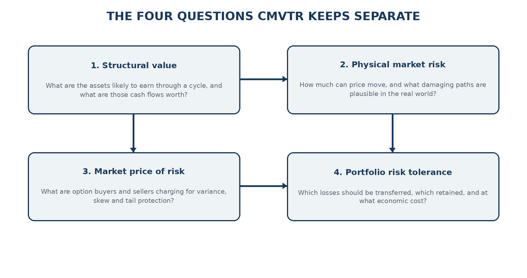
3. Four questions conventional analysis often collapses
Valuation: what are the assets likely to earn through a cycle and what are those cash flows worth today?
Physical risk: how much is the share price likely to move in the real world, and how likely is it to cross a damaging loss barrier before the valuation thesis is realised?
Market price of risk: what are option buyers and sellers charging for variance, downside skew and convexity?
Portfolio policy: which losses are unacceptable, how much insurance carry is tolerable, and how much future upside should be transferred in exchange for protection?
Mixing these questions creates predictable errors. Implied volatility is not the same thing as physical volatility. A low valuation is not proof of low crash risk. Call premium is not free income. A zero-cost collar can still have substantial economic cost.
4. Why methodology is separated from portfolio implementation
A public research framework should be understandable independently of any mandate-specific portfolio implementation. Historical company observations can be used to explain calibration because they are public evidence. Option examples, where useful, should be generic or stylised.
This separation is also a research control. If methodology is designed around a portfolio that already exists, definitions, thresholds and examples can be unconsciously selected to rationalise prior decisions. CMVTR instead fixes the methodology, calibrates it independently and only then permits mandate-specific implementation.
Part II – The CMVTR Framework in Plain English
5. From commodity expectations to structural cash flow
A miner has no single permanent earnings level. Structural earnings are built from the economics of its assets. For each major commodity, CMVTR starts with the price information actually available at the valuation date: spot prices, futures or forward curves where useful, and published longer-horizon forecasts. Historical reconstruction uses archived forecasts rather than realised future prices.
Those expectations are mapped into company-specific realised prices, production volumes, operating costs, royalties, taxes, sustaining capital and growth capital. The objective is Owner Free Cash Flow: cash the asset base can generate after expenditure required to preserve the business, with discretionary growth investment identified separately.
6. Fair value is a distribution
Every major structural input is uncertain. Commodity prices can be wrong. Production can disappoint. Costs can inflate. Capital expenditure can overrun. Currency and discount rates can move. A single fair-value point estimate hides that uncertainty. CMVTR therefore carries structural inputs through a distribution of fair values.
This produces two related valuation variables: magnitude – how far market price is above or below central structural value – and confidence – how much of the fair-value distribution lies clearly on one side of market price.
7. Valuation gap and mean reversion
The valuation gap is the logarithm of market price divided by fair value. A positive gap means price is above the structural centre; a negative gap means below it. CMVTR does not assume the gap closes at a fixed speed. It tests whether overvaluation and undervaluation behave differently and whether convergence changes with commodity trend and volatility regime.
A security can therefore be cheap economically, cheap with valuation confidence, and cheap but still vulnerable because the prevailing state has historically been associated with further deterioration. That third state is particularly important for portfolio timing.
8. Volatility is not one number
CMVTR separates realised physical variation, expected future physical variation, option-implied volatility and downside skew. Realised-volatility research provides the measurement foundation. A Heterogeneous Autoregressive realised-volatility structure, commonly abbreviated HAR-RV, provides a parsimonious baseline for daily, weekly and monthly persistence. Downside semivariance and jumps are treated separately because adverse and discontinuous moves can contain information ordinary variance discards.
9. Yield level and yield shock have different jobs
The United States long-term Treasury yield appears twice for different reasons. The yield level is part of the discount-rate environment applied to predominantly US-dollar mining cash flows. The change in yield is a potential market-risk shock. Separating the two avoids double counting.
10. The option market prices fear; it does not reveal physical probability directly
An option’s implied volatility embeds the market price of bearing uncertainty. It is formed under the risk-neutral pricing measure used to value contingent claims. The investor’s real-world crash probability belongs to the physical measure.
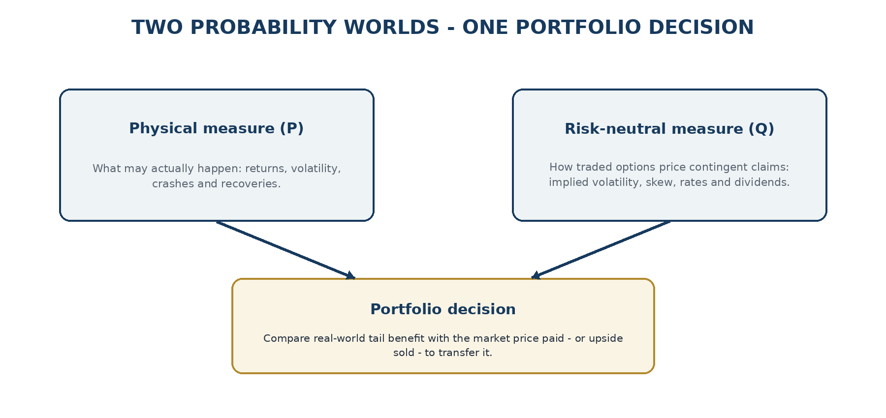
The variance risk premium provides one bridge: option-implied variance minus expected physical realised variance. Downside skew is modelled separately because a crash put buys more than general variance; it buys a disproportionately valuable claim on adverse states.
11. Crash probability is a first-passage problem
CMVTR defines a crash by whether economic wealth touches a loss barrier during the forecast horizon. The principal research target is a 30 per cent barrier within 252 trading days, with 20 and 40 per cent barriers retained to describe the shape of the left tail.
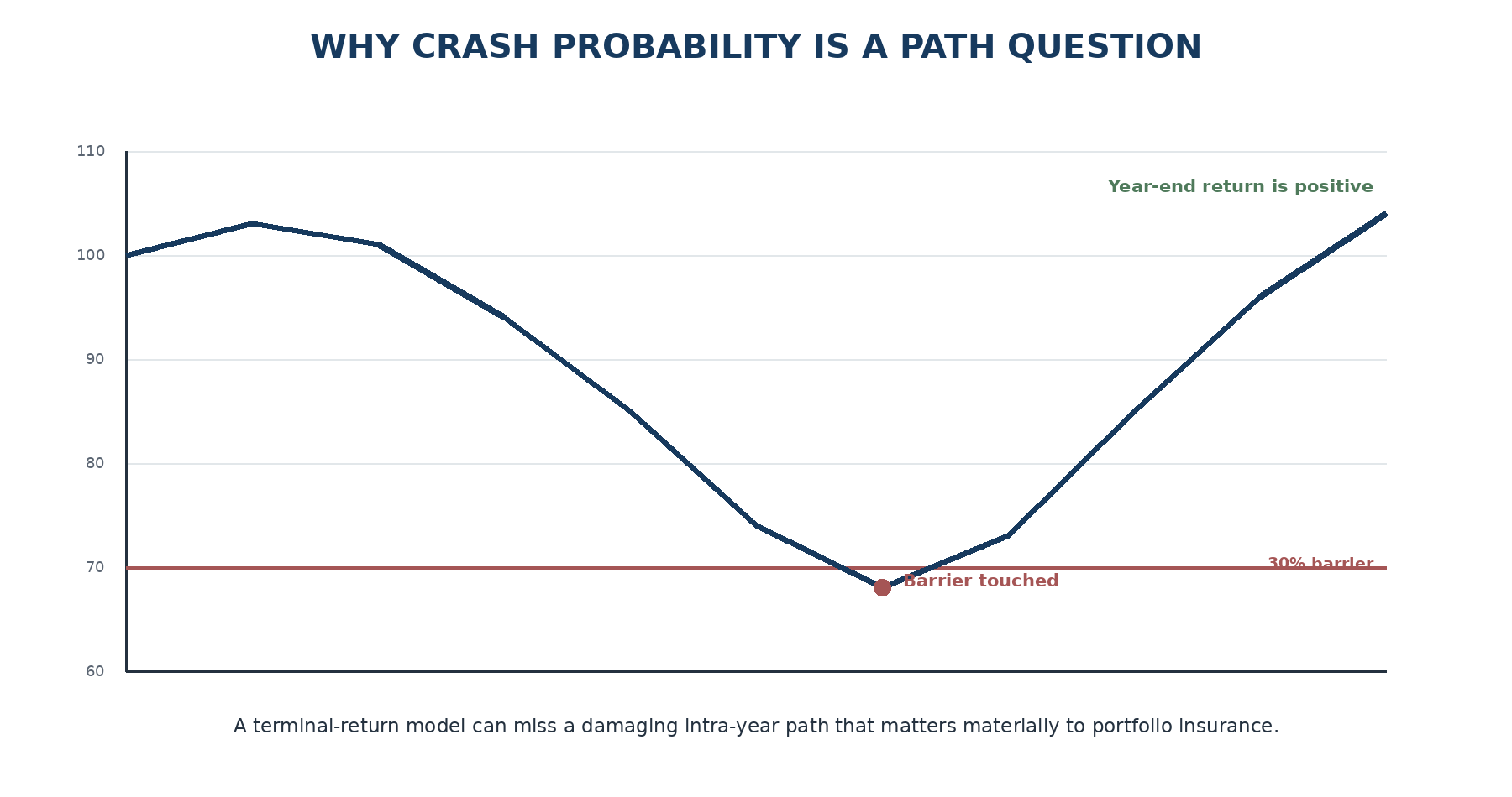
The economic-price series is adjusted for dividends and corporate actions so a mechanical ex-dividend price change is not classified as a crash. The quoted share-price series remains separately available because actual option contracts respond to the quoted underlying and contract-adjustment rules.
12. Why complete paths matter
An option strategy cannot be evaluated from a single terminal stock price. Its economics depend on when the decline occurs, how volatility and skew change during the decline, how much time remains to expiry and whether the stock subsequently recovers. The physical simulation therefore generates complete paths. Options are then valued along those paths using the simulated option surface, rates, dividends and remaining maturity.
13. Buying protection: what makes a put economically efficient?
A put is insurance. Insurance can have negative expected standalone return and still be rational because it pays when the marginal value of cash is unusually high. CMVTR therefore evaluates puts by severe portfolio loss removed per unit of expected economic carry. Expected Shortfall is the primary loss metric.
Expiry is judged against the term structure of crash hazard. A short option may be cheap in upfront cash terms yet cover only a small portion of the modelled twelve-month hazard, while repeated rolling can expose the investor to repricing of insurance after volatility and skew have already risen.
14. Selling upside: why call premium is not free income
A covered call receives cash today by transferring future upside above the strike. The economic question is whether the compensation is adequate for the right-tail wealth surrendered. Linking strike selection to structural value makes the opportunity cost visible, particularly when a security is deeply undervalued and capable of a violent recovery.
15. Why put duration and call duration need not match
The put buys duration of protection. The call sells duration of upside. Those are opposite economic exposures. CMVTR therefore retains as a testable hypothesis that insurance duration can rationally exceed upside-sale duration. A longer-dated put can cover uncertain crash timing; a shorter-dated call can be reconsidered more frequently as valuation changes.
16. From a collar to a dynamic protection architecture
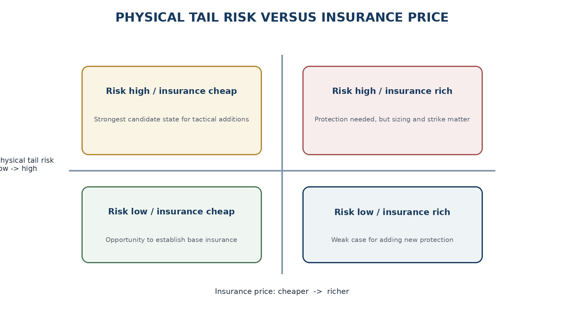
A conventional collar is long stock, long put and short call. CMVTR treats that payoff as one possible state inside a broader dynamic architecture. The put and call are selected independently. Their strikes, maturities and coverage percentages need not match. Base insurance addresses unforecastable shocks and model error; tactical insurance responds to observable risk and the price of protection.
17. Portfolio risk, not position risk
Options are often managed one holding at a time. That can be inefficient when holdings share common tail factors. CMVTR therefore sizes protection using marginal contribution to portfolio Expected Shortfall. A candidate hedge is valued by the reduction in portfolio tail loss it produces per unit of economic cost. Cross-hedging is conceptually permissible where a more liquid or cheaper instrument transfers the common portfolio tail more efficiently, subject to basis risk and mandate constraints.
Part III – Technical Methodology
18. Point-in-time information architecture
Historical model integrity depends more on information timing than on model sophistication. Every prediction date receives an information set containing only data that could reasonably have been known at that date. Each source stores at least an observation date and an availability date. Financial statements enter when released; commodity forecasts when published; company guidance when announced; corporate actions when public.
19. Structural Owner Free Cash Flow engine
Operating cash flow before capital expenditure is built from operating costs, royalties, taxes, working capital and other recurring cash items. Owner Free Cash Flow separates sustaining capital from discretionary growth investment:
The output is a distribution because uncertainty in commodity prices, production, costs, foreign exchange, taxes and capital expenditure is propagated rather than suppressed.
20. Fair-value distribution
Monte Carlo or scenario propagation produces a fair-value distribution. The median and central uncertainty bands are retained.
21. Mean-reversion calibration
Under a stationary simple form, positive kappa implies convergence toward the structural centre. No half-life is assumed in advance. Asymmetry is tested with separate positive and negative valuation-gap terms and a compact state vector of pre-specified regime variables.
22. Realised-volatility model
Candidate extensions include downside realised semivariance, upside semivariance, jump variation, company-specific commodity shocks, market and foreign-exchange factors, yield shocks and valuation interactions. Every extension must improve walk-forward forecast evidence.
23. Expected physical variance, implied variance and the variance risk premium
The physical and option measures are intentionally kept separate. Broad-market evidence motivates the mechanism, but company-specific behaviour must be calibrated from observable option history.
24. First-passage crash hazard
A discrete monthly hazard estimates the conditional probability that the barrier is first crossed in each future month given survival to that point. The predictor vector is deliberately compact: valuation gap and confidence, structural commodity trend and stress, expected physical volatility, downside variation, variance risk premium, put skew, yield shock and one balance-sheet stress measure.
25. Rare-event evidence and overlapping labels
Twelve-month crash labels overlap heavily. One collapse can generate many positive forecast origins; they are not independent crashes. CMVTR therefore reports both labelled origins and distinct underlying crash episodes. Random train/test splits are prohibited. Walk-forward blocks, purge and embargo controls and leave-regime-out challenge tests are used.
26. Joint physical Monte Carlo engine
Fair value evolves with commodity, cost, foreign-exchange, production and discount-rate states. Volatility is endogenous to the path; jumps are separated from continuous innovations; common factor dependence can strengthen under stress. The Monte Carlo engine is constrained by independently calibrated valuation-gap, volatility and first-passage models rather than being permitted to invent its own tail behaviour.
27. Option valuation along physical paths
Physical paths determine what state occurs. Option valuation determines what a traded contingent claim would be worth in that state. At each simulated node, the option engine uses quoted spot, strike, remaining maturity, simulated implied-volatility surface, interest rates, expected dividends and contract exercise style. Contract terms and corporate-action adjustments are part of the model rather than implementation afterthoughts.
28. Put efficiency metrics
A candidate put is described by strike, maturity and hedge quantity. CMVTR measures hazard coverage, protection capture, Expected Shortfall reduction, expected economic carry, roll-repricing risk, liquidity and implementation cost.
No perfect-timing assumption is permitted. A historical strategy must specify in advance whether a put is held to expiry, monetised on a barrier touch, rolled under a pre-specified rule or resized under a pre-specified state trigger.
29. Call efficiency metrics
The covered call’s expected foregone upside is measured path by path against unhedged equity exposure, with particular attention to the right tail and to recovery after a severe drawdown.
30. Dynamic protection optimisation
The optimisation target is not zero net premium. A stylised constrained objective minimises portfolio Expected Shortfall subject to an economic carry budget, minimum right-tail retention, minimum liquidity and maximum turnover. These constraints are governance choices rather than statistical discoveries.
31. Marginal portfolio tail contribution
This shifts optimisation from nominal hedge percentages to the economic question that matters: when the portfolio is genuinely in trouble, which positions and common factors are creating the loss and which instrument transfers that tail most efficiently?
Part IV – Calibration, Validation and Governance
32. Model tournament and the simplest-model rule
Every major component progresses from a simple benchmark to more complex challengers. The production rule is straightforward: choose the simplest model that passes the pre-specified acceptance tests. Sophistication is never an objective in its own right.
33. Historical challenge regimes
| Period | Regime | Primary test |
|---|---|---|
| 2008-09 | Global financial crisis | Tail capacity, stress dependence and large first-passage losses without treating peak earnings as permanent value. |
| 2011-12 | Commodity supercycle peak | Whether very high current cash flow can coexist with lower structural forward expectations. |
| 2015-16 | Mining downturn | Whether trough earnings can be normalised without assuming a cheap share cannot fall further. |
| 2020 | Pandemic shock | Residual shock capacity, volatility feedback, dependence and option repricing. |
| 2020-21 | Rapid recovery / commodity upswing | Whether call overlays preserve enough recovery participation when implied volatility is high and valuation improves. |
34. Point-in-time data governance
Data are classified by authority and by whether they are observed or derived. Primary company filings, exchange data, central-bank series and recognised commodity publications occupy the highest tier. Derived measures maintain explicit lineage. Proxy variables are labelled and receive wider model-risk treatment. Missing data are governed by variable-specific staleness limits rather than silent forward filling.
35. Model risk is part of portfolio risk
Once a quantitative model influences decisions, a portfolio is exposed not only to market risk but to model risk and implementation risk. CMVTR therefore treats intended use, development, validation, monitoring, governance, documentation, inventory, model version and data vintage as components of the investment process.
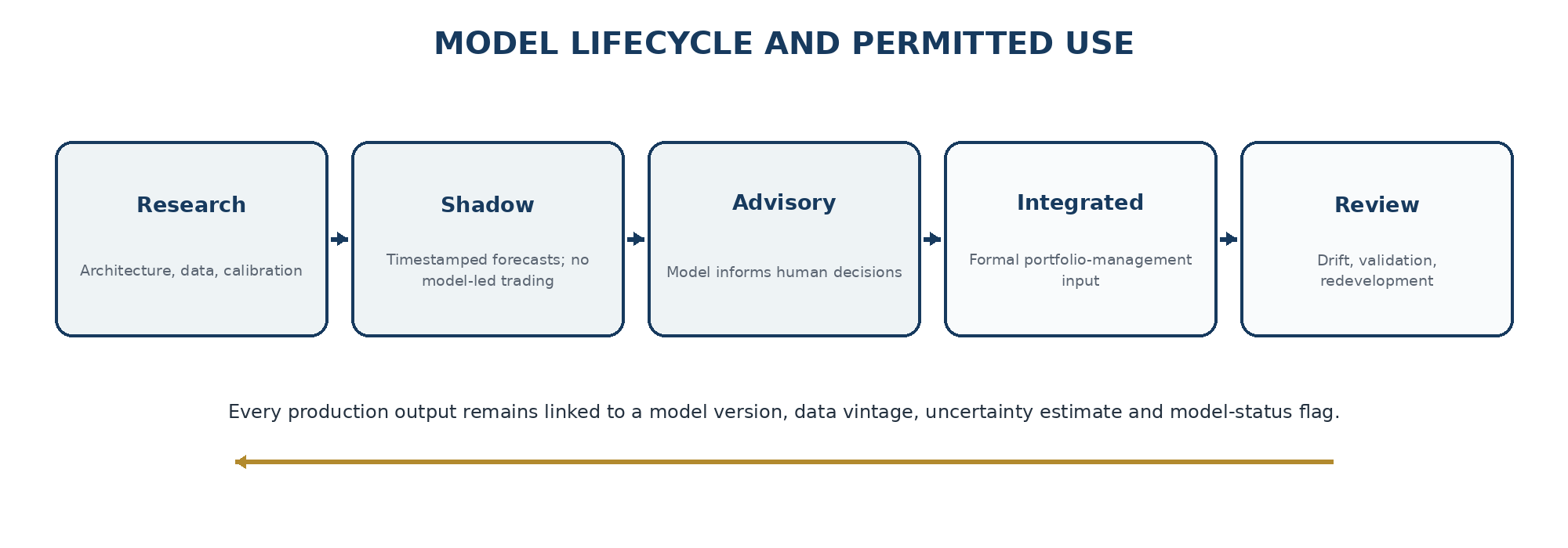
The model-status system is operational: GREEN for normal validated use, AMBER for use with caution and visible uncertainty, and RED where critical data or model failures make normal tactical use inappropriate. A RED model does not imply that the underlying risk has disappeared.
36. Human decision rights
CMVTR is a decision-support system, not an autonomous trading engine. Fundamental research determines whether the business qualifies for ownership. Structural valuation estimates what it is worth. Portfolio construction determines rational exposure. CMVTR then assesses path risk and the economics of transferring that risk. Final implementation remains a human portfolio-management decision under the relevant governance mandate.
Material overrides should be explicit. The system records the model recommendation, the authorised decision and the reason for divergence so that discretion itself can later be evaluated.
37. Shadow deployment before material reliance
During a shadow period, CMVTR should timestamp and store structural fair value, valuation gap, expected physical volatility, crash probabilities, variance risk premium, skew, protection frontiers and model-status flags at each decision date. Forecasts are compared later with realised outcomes but are not rewritten.
A staged use model therefore progresses from Research to Shadow, Advisory and eventually Integrated portfolio use only if evidence warrants increased influence.
38. Limitations
The number of truly independent severe mining crashes is small. Company asset portfolios change through acquisitions, demergers and divestments. Historical option data are shorter and less liquid than equity histories. Commodity expectations are observed imperfectly. Extreme-tail distributions are uncertain. Correlations change in stress. Option-market liquidity and spreads can dominate theoretical value. Human behaviour and policy shocks cannot be fully reduced to the selected variables.
These limitations determine how much influence the model should be allowed to have and how much uncertainty should accompany its outputs. Numerical simulation error can be made very small by increasing path count; model and parameter uncertainty cannot.
39. What is established, what is a Celerity design choice, and what remains a hypothesis
| Topic | Evidence status | CMVTR treatment |
|---|---|---|
| Realised volatility from high-frequency returns | Strong external econometric literature | Established input foundation. |
| HAR multi-horizon volatility persistence | Strong external literature | Baseline candidate model; company performance still calibrated. |
| Downside semivariance contains distinct information | External literature supports asymmetry | Supported candidate extension. |
| Variance risk premium varies through time | Strong broad-market evidence | Company-level behaviour must be calibrated. |
| Valuation predicts future price changes | Broad-market evidence | Motivation only; no imported company coefficient. |
| Valuation improves mining crash prediction | Not established by this methodology paper | Open empirical hypothesis. |
| Longer puts plus shorter calls outperform matched tenors | No generic claim | Open empirical hypothesis subject to net-of-cost historical testing. |
| Post-crash call closure improves recovery capture | Economically plausible | Open empirical hypothesis under pre-specified rules. |
| Portfolio marginal-tail sizing improves protection efficiency | Established portfolio-risk logic; CMVTR implementation is new | Celerity design choice requiring empirical implementation testing. |
40. Implications for portfolio management
A put is not merely a trade on volatility. It is a contract that can convert a discontinuous loss state into cash and liquidity. A short call is not merely yield enhancement. It is a sale of future upside and convexity. A collar is not naturally one indivisible trade; it is a joint decision about two different risk transfers whose appropriate duration and quantity can differ.
Most importantly, a model does not replace portfolio judgement. It creates a common quantitative language in which valuation, risk, option pricing and risk appetite can be discussed without being confused with one another.
41. Research programme from methodology to production
- Reconstruct point-in-time BHP and Rio Tinto structural economics across the historical challenge sample.
- Build fair-value distributions and validate valuation-gap behaviour.
- Assemble long-history and high-frequency volatility datasets and run the volatility model tournament.
- Reconstruct the observable option surface over the reliable exchange-option history.
- Estimate variance-risk-premium and skew behaviour and first-passage crash-hazard models.
- Calibrate the joint Monte Carlo engine against independent volatility and barrier targets.
- Backtest put, call and dynamic protection rules with realistic implementation costs and contract mechanics.
- Freeze the first production model version and commence timestamped shadow forecasts.
- Only after the research framework and evidence are accepted, permit mandate-specific portfolio implementation.
Conclusion – The price of getting from here to value
Traditional fundamental analysis asks what a business is worth. Traditional risk analysis asks how volatile the price is. Option analysis asks what the market is charging for contingent claims. Portfolio construction asks how much loss an investor can tolerate. The error is to assume that one of these questions can stand in for the others.
A low valuation does not prevent a crash. High implied volatility does not reveal the physical probability of that crash. An expensive put can still be economically efficient insurance. A high-premium call can still be an unattractive sale of long-run wealth. A zero-cost collar can still be costly. A sophisticated Monte Carlo can still be wrong.
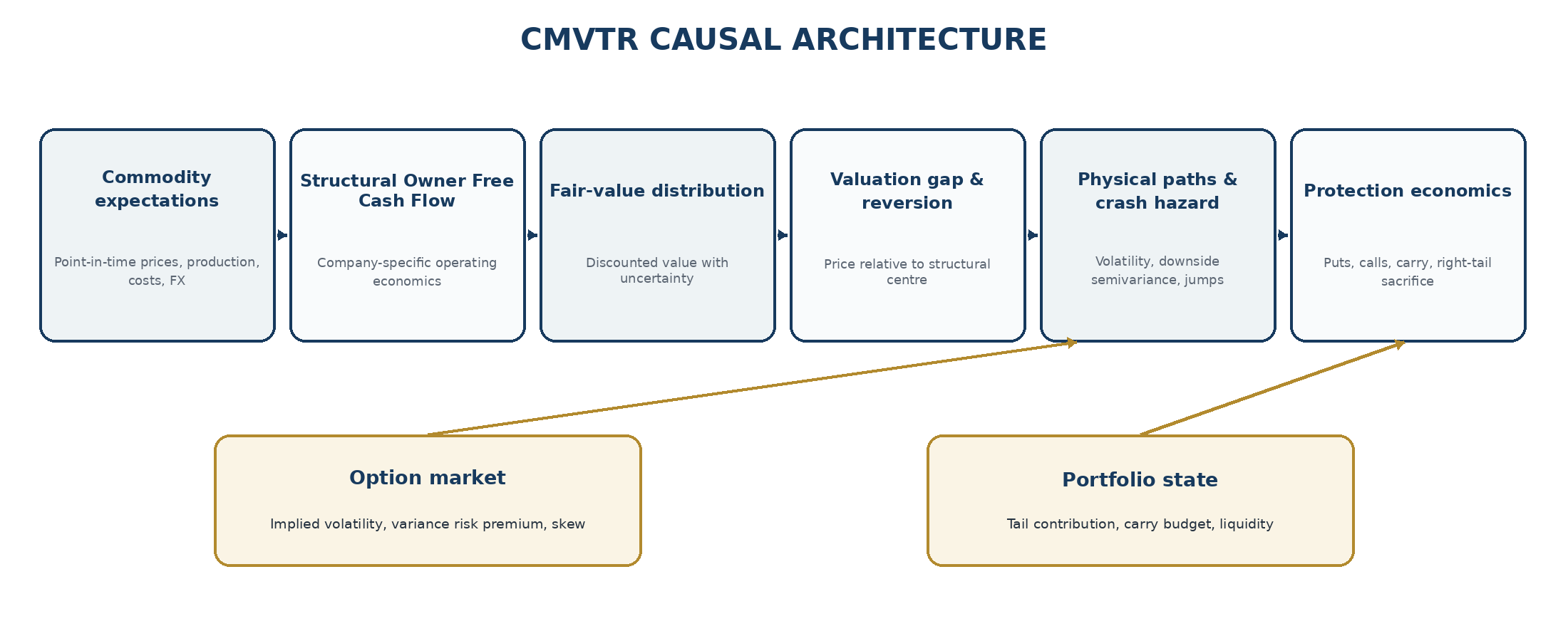
The resulting portfolio question is more demanding: how much is the asset worth, how uncertain is that value, what damaging paths can occur before price and value converge, what is the option market charging to transfer those paths, and how much future upside must be surrendered to finance the transfer?
The Celerity proposition is not that crashes can be forecast perfectly or derivatives can remove risk. It is that valuation, physical risk and the market price of risk can be modelled separately enough to improve the quality of trade-offs between compounding, resilience and liquidity.
Appendix A – Compact Mathematical Specification
Appendix B – Core Variable Dictionary
| Variable | Meaning |
|---|---|
| OwnerFCF | Structural Owner Free Cash Flow after sustaining capital and recurring owner costs. |
| FV50 | Median simulated structural fair value. |
| FVWidth | Width of the central fair-value distribution. |
| VGap | Logarithm of market price divided by median structural fair value. |
| VConf | Confidence measure based on the proportion of fair-value distribution on one side of price. |
| RV | Realised variance. |
| VRP | Variance risk premium: implied variance minus expected physical realised variance. |
| PutSkew | Downside implied volatility relative to at-the-money volatility. |
| CP20 / CP30 / CP40 | Physical first-passage probabilities of touching 20, 30 or 40 per cent economic loss barriers. |
| THE | Tail Hedge Efficiency: Expected Shortfall reduction per unit of expected insurance cost. |
| SUR | Structural Upside at Risk above a written-call strike. |
| MHE | Marginal Hedge Efficiency at portfolio level. |
| ModelStatus | GREEN, AMBER or RED permitted-use flag. |
| DataVintage | Timestamp and version of the point-in-time dataset used for a forecast. |
Appendix C – Historical Challenge Set
The challenge set is not used to demand that the model predict the initiating cause of every crisis. Its role is to test whether the system behaves credibly when confronted with the economic states those episodes created. The pandemic, for example, is a test of residual shock capacity and propagation rather than a claim that a mining model should have forecast a virus.
Appendix D – Data and Model Governance Checklist
| Control | Production requirement |
|---|---|
| Point-in-time information | Observation date and availability date recorded; no future revisions used. |
| Data lineage | Source -> transformation -> intermediate variables -> final output traceable. |
| Corporate actions | Separate economic-wealth and quoted-price treatment; option adjustments recorded. |
| Walk-forward testing | Past predicts genuinely unseen future; random split is not primary evidence. |
| Overlap control | Purge and embargo around overlapping 12-month labels. |
| Rare-event count | Report positive labels and distinct crash episodes. |
| Model tournament | Simplest model that passes; complexity must improve out-of-sample evidence. |
| Uncertainty | Separate Monte Carlo numerical error from model and parameter uncertainty. |
| Version control | Every forecast linked to model version and data vintage; old forecasts never overwritten. |
| Status and fallback | GREEN / AMBER / RED with component-specific fallback rules. |
| Human authority | Model recommendation separated from authorised portfolio decision. |
| Shadow deployment | Timestamp shadow forecasts before material model reliance. |
References and source notes
- Andersen, T.G., Bollerslev, T., Diebold, F.X. and Labys, P. (2003), “Modeling and Forecasting Realized Volatility,” Econometrica, 71(2), 579-625.
- Barndorff-Nielsen, O.E., Kinnebrock, S. and Shephard, N. (2010), “Measuring Downside Risk: Realised Semivariance,” in Volatility and Time Series Econometrics, Oxford University Press.
- Black, F. and Scholes, M. (1973), “The Pricing of Options and Corporate Liabilities,” Journal of Political Economy, 81(3), 637-654.
- Bollerslev, T., Tauchen, G. and Zhou, H. (2009), “Expected Stock Returns and Variance Risk Premia,” Review of Financial Studies, 22(11), 4463-4492.
- Campbell, J.Y. and Shiller, R.J. (2001), “Valuation Ratios and the Long-Run Stock Market Outlook: An Update,” NBER Working Paper 8221.
- Corsi, F. (2009), “A Simple Approximate Long-Memory Model of Realized Volatility,” Journal of Financial Econometrics, 7(2), 174-196.
- Corsi, F., Pirino, D. and Reno, R. (2010), “Threshold Bipower Variation and the Impact of Jumps on Volatility Forecasting,” Journal of Econometrics, 159(2), 276-288.
- Gillis, A., Steen, J., von Nordenflycht, A. and Dunbar, W.S. (2023), “What drives shareholder returns in mining companies?”, Resources Policy, 86, 104217.
- Merton, R.C. (1973), “Theory of Rational Option Pricing,” Bell Journal of Economics and Management Science, 4(1), 141-183.
- Patton, A.J. (2011), “Volatility Forecast Comparison Using Imperfect Volatility Proxies,” Journal of Econometrics, 160(1), 246-256.
- Australian Securities Exchange, equity options contract specifications, equity-derivatives statistics and options education material.
- Board of Governors of the Federal Reserve System, H.15 Selected Interest Rates and model-risk-management guidance.
- Cboe Global Markets, collar-index methodology and benchmark research on protective puts and collars.
- World Bank, Commodity Markets Outlook and Commodity Price Forecast Archive.
CMVTR is a methodology and validation architecture. Company-level empirical claims remain subject to point-in-time calibration, walk-forward testing and model-status controls before greater portfolio influence is permitted.
General information
Celerity publishes general research and commentary only. Nothing in this publication constitutes financial advice, investment advice, personal advice, an offer, solicitation or recommendation to buy or sell any financial product or security.